Data Descriptors (Stats, Relations, Patterns)

Data analysts look for descriptors in data to generate insights.

For a Data aggregator, descriptive attributes of data like size, speed, heterogeneity, lineage, provenance, and usefulness are essential to decide the storage infrastructure scale, data life cycle, and data quality. These aggregator-oriented descriptions are black-box perspectives.

For a Data analyst, descriptive statistics, patterns, and relationships are essential to generate actionable insights. These analyst-oriented descriptions are white-box perspectives. The analysts then use inferential methods to test various hypotheses.

Descriptive Statistics

Data analysts usually work with a significant sample of homogenous records to statistically analyze features. The typical descriptive statistics are – measures of location, measures of center, measures of skewness, and measures of spread.

E.g., A 23 member cricket team of three different states has players of the following ages:

Karnataka: [19,19,20,20,20,21,21,21,21,22,22,22,22,22,22,23,23,23,23,24,24,24,25,25]

Kerala: [19,19,20,20,20,21,21,21,22,22,22,22,23,23,23,23,23,24,24,24,24,24,24]

Maharashtra: [19,19,19,19,19,19,20,20,20,20,20,21,21,21,21,22,22,22,23,23,24,24,25]

Numbers represented this way does not help us detect patterns or explain the data. So, it’s typical to see the tabular distribution view:

AGEKarnatakaKeralaMaharashtra
19226
20335
21434
22543
23452
24362
25201
Age Distribution of State Players

This distribution view is better. So, we would like to see measures of center for this data. These are usually – MEAN, MEDIAN, and MODE.

  • MEAN is the average (Sum Total / # Total)
  • MEDIAN is the middle number
  • MODE is the highest frequency number
MeasureKarnatakaKeralaMaharashtra
MEAN2222.121
MEDIAN222221
MODE222419
Measures of Center

This description is much better. So, we would like to see this graphically to understand the skewness.

Measuring skewness

The age distribution is symmetrical for Karnataka, skewed to the left for Kerala, and skewed to the right for Maharashtra. The data analyst may infer that Karnataka prefers a good mix of ages, Kerala prefers player experience, and Maharashtra prefers the young.

The data analyst may also be interested in standard deviation, i.e., a measure of spread. The standard deviation symbol is sigma (σ) for a sample and is the MEAN distance from the mean value of all values in the sample. Since a distance can be positive or negative, the distance is squared, and the result is square-rooted.

MeasureKarnatakaKeralaMaharashtra
Standard Deviation1.81.71.8
Measure of Spread

In our example, a measure of location (quartiles, percentiles) is also of interest to the data analyst.

PercentileKarnatakaKeralaMaharashtra
25 Percentile212119.5
50 Percentile222221
75 Percentile2323.522
100 Percentile252425
Measure of Location

The table above shows that the 50 percentile value is the median, and the 100 percentile is the maximum value. This location measure is helpful if the values were scores (like in an exam).

Combining statistics and display to explain the data is the art of descriptive statistics. There are several statistics beyond the ones described in this short blog post that could be useful for data analysis.

Time-series Data Patterns

The time-series data has trends, variations and noise.

  1. A trend is the general direction (up, down, flat) in data over time.
  2. Cyclicity variation is the cyclic peaks and troughs in data over time.
  3. Seasonality variation is the periodic predictability of a peak/trough in data.
  4. Noise is meaningless information in data.

The diagrams below provide a visual explanation:

“Ice cream sales are trending upward,” claims an excited ice-cream salesman.

“Used Car value is trending downward,” warns the car salesman

Every business has up and down cycles, but my business is trending upwards,” states a businessman.

It’s the end of the month, so, Salary and EMI season in user accounts, so the transaction volume will be high,” claims the banker.

“There is some white noise in the data,” declared the data scientist.

Data Relationships

Data analysts seek to understand relationships between different features in a data set using statistical regression analysis.

There could be a causal (cause and effect) relationship or simply a correlation. This relationship analysis helps to build predictors.

A simple measure of linear relationship is the correlation coefficient. The measure is not relevant for non-linear relationships. Correlation coefficient of two variables x and y is is calculates as:

correlation(x, y) = covariance(x, y) / (std-dev(x) * std-dev(y))

It’s a number that in the range [-1,1]. Any number closer to zero implies no correlation, and closer to either extremity means higher linear correlation.

  • Negative one (-1) means negatively linearly correlated
  • Positive one (1) means positively linearly correlated
  • Zero (0) means no correlation

Example: Let’s take this random sample.

XYY1Y2Y3
13-383-100
28-8108250
315-15146-50
424-2498150
535-35231-50
648-48220155
763-63170-125
880-80100-150
999-99228-12
10120-120234190
Sample Data
X and YX and Y1X and Y2X and Y3
1-10.60
Correlation coefficient

Visually, we can see that as X increases, Y increases linearly, and Y1 decreases linearly. Hence, the correlation coefficient is positive (1) and negative (-1), respectively. There is no linear relation between X and Y3, and hence, the correlation is 0. The relationship between X and Y2 is somewhere in between with a positive correlation coefficient.

Scatter plot X against (Y, Y1, Y2, Y3)

If X is the number of hours bowler practices and Y2 is the number of wickets, then the correlation between the two can be considered positive.

If X is the number of hours bowler practices and Y3 is the audience popularity score, then the correlation between the two can be considered negligible.

If X is the number of years a leader leads a nation, and Y or Y1 is his popularity index, then the correlation between the two can be considered linearly increasing or decreasing, respectively.

Summary

Data analysts analyze data to generate insights. Insights could be about understanding the past or using the past to predict the (near) future. Using statistics and visualization, the data analysts describe the data and find relationships and patterns. These are then used to tell the story or take actions informed by data.

V’s of Data

Volume, Velocity, Variety, Veracity, Value, Variability, Visibility, Visualization, Volatility, Viability

What are the 3C’s of Leadership? “Competence, Commitment, and Character,” said the wise.

What are the 3C’s of Thinking? “Critical, Creative, and Collaborative,” said the wise.

What are the 3C’s of Marketing? “Customer, Competitors, and Company,” said the wise.

What are the 3C’s of Managing Team Performance? “Cultivate, Calibrate, and Celebrate,” said the wise.

What are the 3C’s of Data? “Consistency, Correctness, and Completeness,” said the wise; “Clean, Current, and Compliant,” said the more intelligent; “Clear, Complete, and Connected,” said the smartest.

“Depends,” said the Architect. Technologists describe data properties in the context of use. Gartner coined the 3V’s – Volume, Velocity, and Variety to create hype around BIG Data. These V’s have grown in volume 🙂

  • 5V’s: Volume, Velocity, Variety, Veracity, and Value
  • 7 V’s: Volume, Velocity, Variety, Veracity, Value, Visualization, and Visibility

This ‘V’ model seems like blind men describing an elephant. A humble engineer uses better words to describe data properties.

Volume: Multi-Dimensional, Size

“Volume” is typically understood in three dimensions. Data is multi-dimensional and stored as bytes—a disk volume stores data of all sizes. Data does not have volume! It has dimensions and size.

A person’s record may include age, weight, height, eye color, and other dimensions. The size of the record may be 24 bytes. When a BILLION person records are stored, the size is 24 BILLION bytes.

Velocity: Speed, Motion

Engineers understand the term velocity as a vector and not a scalar.

A heart rate monitor may generate data at different speeds, e.g., 82 beats per minute. I can’t say my heart rate is 82 beats per minute to the northwest. Hence, heart rate is a speed. It’s not heart velocity. I can say that a car is traveling 35 kilometers per hour to the northwest. The velocity of the vehicle is 35KMPH NW.

Data does not have direction; hence it does not have velocity. Data in motion has speed.

Variety: Heterogeneity

The word variety is used to describe differences in an object type, e.g., egg curry varieties, pancake varieties, sofa varieties, tv varieties, image data format varieties (jpg, jpeg, bmp), and data structure varieties (structured, unstructured, semi-structured). Data variety is abstract and is a marketecture term.

Heterogeneity is preferred because it explicitly states that:

  1. Data has types (E.g., String, Integer, Float, Boolean)
  2. Composite types are created by composing other data types (E.g., A Person Type)
  3. Composite types could be structured, unstructured, or semi-structured (E.g., A Person Type is semi-structured as the person’s address is a String type)
  4. Collections contain the same or different data types.
  5. Types, Composition, and Collections apply to all data (BIG or not).

Veracity: Lineage, Provenance

Veracity means Accurate, Precise, and Truthfulness.

Let’s say that a weighing scale reports the weight of a person as 81.5 KG. Is this accurate? Is the weighing scale calibrated? If the same person measures her weight on another weighing scale, the reported weight might be 81.45 KG. The truth may be 81.455 KG.

Data represent facts, and when new facts are available, the truth may change. Data cannot be truthful; it’s just facts. Meaning or truthfulness is derived using a method.

Lineage and provenance meta-data about Data enables engineers’ to decorate the fact with other useful facts:
1. Primary Source of Data
2. Users or Systems that contributed to Data
3. Date and Time of Data collection
4. Data creation method
5. Data collection method

Value: Useful

If Data is a bunch of facts, how can it be valuable? Understandably, the information generated from data by analyzing the facts is valuable. Data (facts) can either be useful to create valuable information or useless and discarded. We associate a cost to a brick and a value to a house. Data is like bricks used to build valuable information/knowledge.

Summary

I did not go into every V, but you get the drill. If an interviewer asks you about 5V’s in an interview, I request you to give the standard marketecture answer for their sanity. The engineer’s vocabulary is not universal; technical journals publish articles in the sales/marketing vocabulary. As engineers/architects, we have to remember the fundamental descriptive properties of data so that the marketecture vocabulary does not fool us. However, we have to internalize the marketecture vocabulary and be internally consistent with engineering principles.

It’s not a surprise that Gartner invented the hype cycle.

Data Aggregation (Map, Filter, Reduce)

Data engineers think in batches!

Thinking in batches reminds me of a famous childhood story.

Once upon a time, a long, long time ago, there was a kind and gentle King. He ruled people beyond the horizon, and his subjects loved him.

One day, a tired-looking village man came to the King and said, “Dear King, help us. I am from a village beyond the horizon. It’s been raining for several days. My village chief asked me to fetch help from you before disaster strikes. It took me five days to walk to the Kingdom, and I am tired but glad that I could deliver this message to you.”

“I am glad that you came for help. I will send Suppandi, my loyal Chief of Defence, to assess the damage and then send help,” said the King. “Suppandi, you have your orders. Now, go. Assess the damage, report to me, and help,” ordered the King.

Suppandi left to the village beyond the horizon on his fastest horse. When he reached the town, the town was flooded, and Suppandi felt the urge to return to the King quickly to inform him about the floods. So, he drove his horse faster and reached the Kingdom in 1/2 day. He went to the King and told him. “Dear King, the village is flooded. I went in a day and came back in 1/2 day to give you this information.”

Suppandi was pleased with himself. However, the King wanted more information. “Suppandi, please tell me whether people in the village have food, are children hurt? What can we do more to help?”

“I will find out, Dear King,” said Suppandi. He left again on his fastest horse. This time he reached in 1/2 day. He figured that people don’t have food, and many children are hurt and homeless. He raced back to the Kingdom. “Dear King, I reached in 1/2 day and came back in another 1/2. The villagers don’t have food to eat, and they are hungry. Several children are hurt and need medical attention,” said Suppandi.

This time the King had more questions. “Dear Suppandi, what did the village chief say? What can we do for him?”

“Dear King, I will find out. Let me leave to the village immediately,” said Suppandi.

Chanakya was eagerly listening in to the conversation. He told Suppandi, “Dear Suppandi, you must be tired. Let me take over. Take some rest.”

Immediately, Chanakya ordered his men to collect food, water, clothes, medicines, and doctors. He asked for the fastest horses, and along with several men and doctors, he left for the village beyond the horizon. When he reached, the town was flooded, and people were on their home terraces. He found several houses destroyed and hungry kids taking shelter under the trees, and many wounded villagers.

He ordered his men to save the villagers skirting the flood, protect all children, feed them, and take them to a safe place. He also called the doctors to attend to the wounds.

The men built a temporary home outside the village to give shelter to the homeless. They waited for a few days for the rain and flood to subside. When it was bright and sunny, Chanakya, his men, and the villagers cleaned the village, re-built the homes, and deposited enough food and grains for six months before saying goodbye.

Chanakya reached the Kingdom and immediately reported to the King. The King was anxious. He said, “Chanakya, you were gone for two weeks with no message from you. I was worried. Did you speak to the village Chief?”

“Dear King, Yes, on your behalf, I spoke to the village chief. I found that the village was flooded, so we rescued all the villagers, attended to the wounded, fed them, re-built their homes, and left food and grains for six months. The people have lost their belongings in flood, but all of them are safe, and they have sent their wishes and blessings for your timely help,” said Chanakya.

The King was pleased. “Chanakya, I should have sent you earlier. You are a batch thinker! Thank you,” said the King.

Suppandi was disappointed. He had worked hard to drive to the village and report to the King as instructed, but Chanakya gets all the praises. To this date, he still does not understand and is hurt.

Most non-data engineers are like Suppandi; they use programming constructs like “for,” “if,” “while,” and “do” on remote data. Most data engineers are like Chanakya; they use the programming constructs like “map,” “filter,” “reduce,” and “forEach.” Programming with data is always functional/declarative, while traditional programming is imperative.

There is nothing wrong with acting like Suppandi; he is the Chief of Defence. But, some cases require Chanakya thinking. In architectural language, Suppandi actions move data to algorithms, and Chanakya actions move algorithms to data. The latter works better when there is a distance and cost-to-travel between data and algorithms.

This difference in thinking is why data engineers use SQL, and traditional engineers use C#/Java. SQL uses declarative commands that are sent to the database to pipeline a set of actions on data. The conventional programming languages have caught up to the declarative programming paradigm by supporting lambda functions (arrow functions), and map/filter/reduce style functions on data collections. The map/filter/reduce style functions allow compilers/interpreters to leverage the underlying parallel compute backbone (the expensive eight-core CPU) or use a set of inexpensive machines for parallel computing. They are abstracting away parallelism from the programmer. The programmer helps the compiler/interpreter to identify speed-improvement opportunities by explicitly programming declaratively.

Mapping

Instead of iterating over a collection one at a time, a map is a function to apply another function to all elements of a collection. The map function may split the collection into parts to distribute to different cores/machines. The underlying collection remains immutable. In general, mapping could mean one-2-one, one-2-many, and many-2-one; and is the process of applying a relation (function) to map an element in the domain with an element in the range. In the case of computing, mapping does not change the size of the collection.

E.g., [1,2,-1,-2] => [1,4,1,4] using the squared relation is a many-2-one mapping

var numbers = [1, 2, -1, -2];
var x = numbers.map(x => x ** 2);
console.log(x);
[1,4,1,4]

E.g., [1,2,-1,-2] => [2,3,0,-1] using the plus one relation is a one-2-one mapping

var numbers = [1, 2, -1, -2];
var x = numbers.map(x => x + 1);
console.log(x);
[2, 3, 0, -1]

E.g., [1,2,-1,-2] using the plus one and squared relation is a one-2-many mapping

var numbers = [1, 2, -1, -2];
var x = numbers.map(x => [x + 1, x ** 2]);
console.log(x);
[[2, 1], [3, 4], [0, 1], [-1, 4]]

E.g., An SQL Example of a one-2-one mapping

SELECT Upper(ContactName)
FROM Customers
MARIA ANDERS
ANA TRUJILLO
ANTONIO MORENO
THOMAS HARDY

Filtering

Instead of iterating over a collection one at a time, a filter is a function to return a subset of elements that match criteria. The filter function may split the collection into parts to distribute to different cores/machines. The underlying collection remains immutable. Examples:

var numbers = [1, 2, -1, -2];
var x = numbers.filter(x => x > 0);
console.log(x);
[1, 2]
SELECT *
FROM Customers
WHERE Country="USA"

Number of Records: 13

CustomerIDCustomerNameContactNameAddressCityPostalCodeCountry
32Great Lakes Food MarketHoward Snyder2732 Baker Blvd.Eugene97403USA
36Hungry Coyote Import StoreYoshi LatimerCity Center Plaza 516 Main St.Elgin97827USA
43Lazy K Kountry StoreJohn Steel12 Orchestra TerraceWalla Walla99362USA
45Let’s Stop N ShopJaime Yorres87 Polk St. Suite 5San Francisco94117USA

Reduce

Instead of iterating over a collection one at a time, a reduce is a function to return a single value. The reduce function may split the collection into parts to distribute to different cores/machines. The underlying collection remains immutable. Examples:

var numbers = [1, 2, -1, -2];
var x = numbers.reduce((sum,x) => sum + x, 0);
console.log(x);
0
SELECT count(*)
FROM Customers
Number of Records: 1
count(*)
91

Pipelining

When multiple actions need to be performed on the data then it’s a norm to pipeline the actions. Examples:

var numbers = [1, 2, -1, -2];
var x = numbers
  .map(x => x + 1) //[2,3,0,-1]
  .filter(x => x > 0) //[2,3]
  .map(x => x ** 2) //[4,9]
  .reduce((sum, x) => sum + x, 0) //13
console.log(x);
13
SELECT Country, Upper(Country), count(*)
FROM Customers
WHERE Country LIKE "A%"        
GROUP BY Country
Number of Records: 2
Country Upper(Country) count(*)
Argentina ARGENTINA 3
Austria AUSTRIA 2

Takeaway

Data Engineers use Chanakya thinking to get work done in batches. Even streaming data is processed in mini-batches (windows). Actions on data are pipelined and expressed declaratively. The underlying compiler/interpreter abstracts away parallel computing (single device, multiple devices) from the programmer.

Think in Batches for Data.

Data Quality (Dirty vs. Clean)

Data Quality has a grayscale, and data quality engineers can continually improve data quality. Continual quality improvement is a process to achieve data quality excellence.

Dirty data may refer to several things: Redundant, Incomplete, Inaccurate, Inconsistent, Missing Lineage, Non-analyzable, and Insecure.

  • Redundant: A Person’s address data may be redundant across data sources. So, the collection of data from these multiple data sources will result in duplicates.
  • Incomplete: A Person’s address record may not have Pin Code (Zip Code) information. There could also be cases where the data may be structurally complete but semantically incomplete.
  • Inaccurate: A Person’s address record may have the wrong city and state combination (E.g., [City: Mumbai, State: Karnataka], [City: Salt Lake City, State: California])
  • Inconsistent: A Person’s middle name in one record is different from the middle name in another record. Inconsistency happens due to redundancy.
  • Missing Lineage (and Provenance): A Person’s address record may not reflect the current address as the user may not have updated it. It’s an issue of freshness.
  • Non-analyzable: A Person’s email record may be encrypted.
  • Insecure: A Person’s bank account number is available but not accessible due to privacy regulations.

The opposite of Dirty is Clean. Cleansing data is the art of correcting data after it is collected. Commonly used techniques are enrichment, de-duplication, validation, meta-information capture, and imputation.

  1. Enrichment is a mitigation technique for incomplete data. A data engineer enriches a person’s address record by adding country information by mapping the (city, state) tuple to a country.
  2. De-Duplication is a mitigation technique for redundant data. The data system identifies and drops duplicates using data identities. Inconsistencies caused by redundancies require use-case-specific mitigations.
  3. Validation is a mitigation technique that applies domain rules to verify correctness. An email address can be verified for syntactical correctness by using a regular expression (\A[\w!#$%&’+/=?{|}~^-]+(?:\.[\w!#$%&'*+/=?{|}~^-]+)@(?:[A-Z0-9-]+.)+[A-Z]{2,6}\Z). Data may be accepted or rejected based on validations.
  4. Lineage and Provenance capture is a mitigation technique for data where source or freshness is critical. An image grouping application will require meta-data about an image series (video) collected like phone type and captured date.
  5. Imputation is a mitigation technique for incomplete data (data with information gaps due to poor collection techniques). A heartrate time-series data may be dirty with missing data in minutes 1 and 12. Using data with holes may lead to failures, so a data imputation may use the previous or next value to fill the gap.

These are cleansing techniques to reduce data dirtiness after data is collected. However, data dirtiness originates at creation time, collection time, and correction time. So, a data cleansing process may not always result in non-dirty data.

A great way to start with data quality is to describe the attributes of good quality data and related measures. Once we have a description of good quality data, incrementally/iteratively use techniques like CAPA (corrective action, preventive action) with a continual quality improvement process. Once we are confident about data quality given current measures, the data engineer can introduce new KPIs or set new targets for existing ones.

Example: A research study requires collecting stroke imaging data. A description of quality attributes would be:

Data Quality AttributeDescription
Data Lineage & Provenance– Countries: {India}
– Imaging Types: {CT}
– Source: {Stroke Centers, Emergency}
– Method – Patient Position: supine
– Method – Scan extent: C2-2-vertex
– Method – Scan direction: caudocranial
– Method – Respiration: suspended
– Method – Acquisition-type: volumetric
– Method – Contrast: {Non-contrast CT, PCT with contrast}
RedundancyMultiple scans of the same patient are acceptable but need to be separated by one week.
CompletenessEach imaging scan should be accompanied by a radiology report that describes these features of the stroke:
– Time from onset: { early hyperacute (0-6H), late hyperacute (6-24H), acute (1-7D), sub-acute (1-3W), chronic (3W+) }
– CBV (Cerebral Blood Volume) in ml/100g of brain tissue
– CBF (Cerebral Blood Flow) in ml/min/100g of brain tissue
– Type of Stroke: {Hemorrhagic-Intracerebral, Hemorrhagic-subarachnoid, Ischemic-Embolic, Ischemic-Thrombotic}
AccuracyThree reads of the image by separate radiologists to circumvent human errors and bias. Anonymized Patient history is sent to the radiologist.
Security and PrivacyPatient PII is not leaked to the radiologist interpreting the result or the researcher analyzing the data.
Data Quality Attributes

As you can see from the table of attributes for CT Stroke imaging data, the quality description is data-specific and use-specific.

Data engineers compute attribute-specific metrics using data attribute descriptions on a data sample to measure overall data quality. These attribute descriptions are the N* to pursue excellence in data quality.

Summary: The creation, collection, and correction improve over some time when measured using criteria. There will always be data quality blind spots and leakages. Hence, data engineers report data quality on a grayscale with multiple attribute-specific metrics.

Streaming vs. Messaging

We already have pub/sub messaging infrastructure in our platform. Why are you asking for a streaming infrastructure? Use our pub/sub messaging infrastructure” – Platform Product Manager

Streaming and Messaging Systems are different. The use-cases are different.

Both streaming and messaging systems use the pub-sub pattern with producers posting messages and consumers subscribing. The subscribed consumers may choose to poll or get notified. Consumers in streaming systems generally poll the brokers, and the brokers push messages to consumers in messaging systems. Engineers use streaming systems to build data processing pipelines and messaging systems to develop reactive services. Both systems support delivery semantics (at least once, exactly once, at most once) of the messages. Brokers in streaming systems are dumber than messaging systems that build routing and filtering intelligence in the brokers. Streaming systems are faster than messaging systems due to a lack of routing and filtering intelligence 🙂

Let’s look at the top three critical differences in detail:

#1: Data Structures

In streaming, the data structure is a stream, and in messaging, the data structure is a queue.

Queue” is FIFO (First In First Out) data structure. Once a consumer consumes an element, it is removed from the queue, reducing the queue size. A consumer cannot fetch the “third” element from the queue. Queues don’t support random access. E.g., A queue of people waiting to board a bus.

Stream” is a data structure that is partitioned for distributed computing. If a consumer reads an element from a stream, the stream size does not reduce. The consumer can continue to read from the last read offset within a stream. Streams support random access; the consumer may choose to seek any reading offset. The brokers managing streams keep the state of each consumer’s reading offset (like a bookmark while reading a book) and allow consumers to read from the beginning, the last read offset, a specific offset, or the latest. E.g., a video stream of movies where each consumer resumes at a different offset.

In streaming systems, consumers refer to streams as Topics. Multiple consumers can simultaneously subscribe to topics. In messaging systems, the administrator configures the queues to send messages to one consumer or numerous consumers. The latter pattern is called a Topic used for notifications. A Topic in the streaming system is always a stream, and it’s always a queue in a messaging system.

Both stream and queue data structures order the elements in a sequence, and the elements are immutable. These elements may or may not be homogenous.

Queues can grow and shrink with publishers publishing and consumers consuming, respectively. Streams can grow with publishers publishing messages and do not shrink with consumers consuming. However, streams can be compacted by eliminating duplicates (on keys).

#2: Distributed (Cluster) Computing Topology

Since a single consumer consumes an element in a queue in a load-balancing pattern, the fetch must be from the central (master) node. The consumers may be in multiple nodes for distributed computing. The administrator configures the master broker node to store and forward data to other broker nodes for resiliency; however, it’s a single master active-passive distributed computing paradigm.

In the notification (topic) pattern, multiple consumers on a queue can consume filtered content to process data in parallel. The administrator configures the master node to store and forward data to other broker nodes that serve consumers. The publishers publish to a single master/leader node, but consumers can consume from multiple nodes. This pattern is the CQRS (Command Query Responsibility Segregation) pattern of distributing computing.

The streaming pattern is similar to the notification pattern w.r.t. distributed computing. Unlike messaging, partition keys break streams into shards/partitions, and the lead broker replicates these partitions to other brokers in the cluster. The leader election process selects a broker as a leader/master for a given shard/partition, and shard/partition replications serve multiple consumers in the CQRS pattern. The consumers read streams from the last offset, random offset, beginning, or latest.

If the leader fails, either a passive slave can take over, or the cluster elects a new leader from existing slaves.

#3: Routing and Content Filtering

In messaging systems, the brokers implement the concept of exchanges, where the broker can route the messages to different endpoints based on rules. The consumers can also filter content delivered to them at the broker level.

In streaming systems, the brokers do not implement routing or content filtering. Consumers may filter content, but utility libraries in the consumer filter out the content after the broker delivers the content to the consumer.

Tabular Differences View

CategoryStreamingMessaging
Support Publish and Subscribe ParadigmYesYes
Polling vs. NotificationPolling by ConsumersNotification by Brokers to consumers
Use CaseData Processing PipelinesReactive (micro)services
Delivery Semantics Supportedat-most-once
at-least-once
exactly-once
at-most-once
at-least-once
exactly-once
Intelligent BrokerNoYes
Data StructureStreamQueue
PatternsCQRSContent-Based Routing/Filtering
Worker (LB) Distribution
Notification
CQRS
Data ImmutabilityYesYes
Data RetentionYes. Not deleted after delivery.No. Deleted after delivery.
Data compactionYes. Key de-duplication.N/A
Data HomogeneityHeterogenous by Default. Supports schema checks on data outside the broker.Heterogenous by Default.
SpeedFaster than MessagingSlower than Streaming
Distributed Computing TopologyBroker cluster with single master per stream partition and consumers consuming from multiple brokers with data replicated across brokersBroker cluster with single master per topic/queue. Active-passive broker configuration for the load-balancing pattern. Data replicated across brokers for multiple consumer distribution.
State/MemoryBrokers remember the consumers’ bookmark (state) in the streamConsumers always consume from time-of-subscription (latest only)
Hub-and-Spoke ArchitectureYesYes
Vendors/Services (Examples)Kafka
Azure Event Hub
AWS Kinesis
RabbitMQ
Azure Event Grid
AWS SQS/SNS
Domain ModelA stream of GPS positions of a moving carA queue to buy train tickets
Table of Differences between Streaming/Messaging Systems

Visual Differences View

Summary

Use the right tool for the job. Use messaging systems for event-driven services and streaming systems for distributed data processing.

Data Batching, Streaming and Processing

The IT industry likes to treat data like water. There are clouds, lakes, dams, tanks, streams, enrichments, and filters.

Data Engineers combine Data Streaming and Processing into a term/concept called Stream Processing. If data in the stream are also Events, it is called Event Stream Processing. If data/events in streams are combined to detect patterns, it is called Complex Event Processing. In general, the term Events refers to all data in the stream (i.e., raw data, processed data, periodic data, and non-periodic data).

The examples below help illustrate these concepts:

Water Example:

Let’s say we have a stream of water flowing through our kitchen tap. This process is called water streaming.

We cannot use this water for cooking without first boiling the water to kill bacteria/viruses in the water. So, boiling the water is water processing.

If the user boils the water in a kettle (in small batches), the processing is called Batch Processing. In this case, the water is not instantly usable (drinkable) from the tap.

If an RO (Reverse Osmosis) filtration system is connected to the plumbing line before the water streams out from the tap, it’s water stream processing with filter processors. The water stream output from the filter processors is a new filtered water stream.

A mineral-content quality processor generates a simple quality-control event on the RO filtered water stream (EVENT_LOW_MAGNESIUM_CONTENT). This process is called Event Stream Processing. The mineral-content quality processor is a parallel processor. It tests several samples in a time window from the RO filtered water stream before generating the quality control event. The re-mineralization processor will react to the mineral quality event to Enrich the water. This reactive process is called Event-Driven Architecture. The re-mineralization will generate a new enriched water stream with proper levels of magnesium to prevent hypomagnesemia.

Suppose the water infection-quality control processor detects E-coli bacteria (EVENT_ECOLI), and the water mineral-quality control processor detects low magnesium content (EVENT_LOW_MAGNESIUM_CONTENT). In that case, a water risk processor will generate a complex event combining simple events to publish that the water is unsuitable for drinking (EVENT_UNDRINKABLE_WATER). The tap can decide to shut the water valve reacting to the water event.

Water Streaming and Processing generating complex events

Data Example:

Let’s say we have a stream of images flowing out from our car’s front camera (sensor). This stream is image data streaming.

We cannot use this data for analysis without identifying objects (person, car, signs, roads) in the image data. So, recognizing these objects in image data is image data processing.

If a user analyses these images offline (in small batches), the processing is called Batch Processing. In the case of eventual batch processing, the image data is not instantly usable. Any events generated from such retrospective batch processing are too late to react.

If an image object detection processor connects to the image stream, it is called image data stream processing. This process creates new image streams with enriched image meta-data.

If a road-quality processor generates a simple quality control event that detects snow (EVENT_SNOW_ON_ROADS), then we have Event Stream Processing. The road-quality processor is a parallel processor. It tests several image samples in a time window from the image data stream before generating the quality control event.

Suppose the ABS (Anti-lock Braking Sub-System) listens to this quality control event and turns on the ABS. In that case, we have an Event-Driven Architecture reacting to Events processed during the Event Stream Processing.

Suppose the road-quality processor generates snow on the road event (EVENT_SNOW_ON_ROAD), and a speed-data stream generates vehicle speed data every 5 seconds. In that case, an accident risk processor in the car may detect a complex quality control event to flag the possibility of accidents (EVENT_ACCIDENT_RISK). The vehicle’s risk processor performs complex event processing on event streams from the road-quality processor and data streams from the speed stream. i.e., by combining (joining) simple events and data in time windows to detect complex patterns.

Data Streaming and Processing generating complex actionable events

Takeaway Thoughts

As you can see from the examples above, streaming and processing (Stream processing) is more desired than batching and processing (Batch processing) because of actionable real-time event generation capability.

Data engineers define data-flow “topology” for data pipelines using some declarative language (DSL). Since there are no cycles in the data flow, the pipeline topology is a DAG (Directed Acyclic Graph). The DAG representation helps data engineers visually comprehend the processors (filter, enrich) connected in the stream. With a DAG, the operations team can also effectively monitor the entire data flow for troubleshooting each pipeline.

Computing leverages parallel processing at all levels. Even with small data, at the hardware processor level, clusters of ALU (Arithmetic Logic Unit) process data streams in parallel for speed. These SIMD/MIMD (Single/Multiple Instruction Multiple Data) architectures are the basis for cluster computing that combines multiple machines to execute work using map-reduce with distributed data sets. The BIG data tools (E.g., Kafka, Spark) have effectively abstracted cluster computing behind common industry languages like SQL, programmatic abstractions (stream, table, map, filter, aggregate, reduce), and declarative definitions like DAG.

We will gradually explore big data infrastructure tools and data processing techniques in future blog posts.

Data stream processing is processing data in motion. Processing data in motion helps generate real-time actionable events.

Data Semantics

The real world is uncertain, inconsistent, and incomplete. When people interact with the real world, data from their inbuilt physical sensors (eyes, ears, nose, tongue, skin) and mental sensors (happiness, guilt, fear, anger, curiosity, ignorance, and many more) get magically converted into insights and actions. Even if these insights are shared & common, the actions may vary across people.

Example: When a child begs for money on the streets, some people choose to give money, others prefer to ignore the child, and some others decide to scold the child. These people have a personal biased context overlooking the fact that it’s a child begging for money (or food), and their actions result from this context.

The people who give money claim that they feel sorry for the child, and parting away little money won’t damage them and help the child eat. The people who don’t give money argue that giving cash would encourage more begging, and a mafia runs it. Some people may genuinely have no money, and others expect the governments (or NGOs) to step up.

Switching context to the technology world:

With IoT, Cloud, and BIG Data technologies, everybody wants to collect data, get insights, and convert these insights into actions for business profitability. This computerized data and workflow automation system approximates an uncertain, inconsistent, and incomplete real-world setup. Call this IoT, Asset Performance Management (APM), or a Digital Twin; the data to insights to actions process is biased. Automating a biased process is a hard problem to solve.

It’s biased because of semantics of the facts involved in the process.

semantics [ si-man-tiks ]

“The meaning, or interpretation of the meaning, of a fact or concept”

Semantics is to humans as syntactic is to machines. So, a human in the loop is critical to manage semantics. AI is changing the human-in-the-loop landscape but comes with learning bias.

Let’s try some syntactic sugar to decipher semantics.

Data Semantics, Data Application Semantics

Data semantics is all about the meaning, use, and context of Data.

Data Application Semantics is all about the meaning, use, and context of Data and application agreements (contracts, methods).

Sounds simple? Not to me. I had to read that several times!

Let’s dive in with some examples:

Example A: A Data engineer claims: “My Data is structured (quantifiable with schema). So, AI/BI applications can use my Data to generate insights & actions”. Not always true. Mostly not.

Imagine a data structure that captures the medical “heart rate” observation. The structure may look like {“rate”: 180, “units”: ‘bpm’} with a schema that defines the relevant constraints (i.e., the rate is a mandatory field and must be a number >=0 expressed as beats per minute).

An arrhythmia detection algorithm, analyzing this data structure might send out an urgent alarm – “HELP! Tachycardia”, and dial 102 to call an ambulance. The ambulance arrives to find that the person was running on a treadmill, causing a high heart rate. This Data is structured but “incomplete” for analysis. The arrhythmia detection algorithm will need more context than the rate and units to raise the alarm. It will need context to “qualify” and “interpret” the “heart-rate” values. Some contextual data elements could be:

  1. Person Activity: {sleeping, active, very active}
  2. Person Type: {fetal, adult}
  3. Persons age: 0-100
  4. Measurement location: {wrist, neck, brachial, groin, behind-knee, foot, abdomen}
  5. Measurement type: {ECG, Oscillometry, Phonocardiograpy, Photoplethysmography}
  6. Medications-in-use: {Atropine, OTC decongestants, Azithromycin, …}
  7. Location: {ICU, HDU, ER, Home, Ambulance, Other}

Let’s look at this example from the “semantics” definition above:

  1. The meaning of “heart rate” is abstract but consistently understood as heart contractions per minute.
  2. The “heart rate” observation is used to build an arrhythmia detection application.
  3. Additional data context required to interpret “heart-rate” is Activity, Person Type, Person Age, Measurement Location, Measurement Type, Medications-in-use, and Location. This qualifying context is use-specific. An application to identify the average heart-rate range in a population by age intervals needs only the Person Age.
  4. The algorithm’s agreement (contract = what?) is to “Detect arrhythmias and Call Ambulance in case of ER care”
  5. The algorithm’s agreement (method = how?) is not well defined. A competing algorithm may use AI to make a better prediction to avoid false alarms. This is similar to our beggar child analogy, where the method of the people to derive insight differed, resulting in different actions.

Example B: Another familiar analogy to help understand “meaning,” “use,” “context,” and “agreement” is to look at food cooking recipes. Almost all these recipes have the statement “add salt to taste.”

  • The meaning of “Salt” is abstract but consistent. Salt is not sugar! 🙂 It’s salt.
  • Salt is used to make the food tasty.
  • Additional data context required to interpret “Salt” is the salt-type {pink salt, black salt, rock salt, sea salt}, users salt toleration level {bland, medium, saltier}, users BP, and users-continent {Americas, Asia, Europe, Africa, Australia}.
  • The agreement (contract = what?) is to “Add Salt.”
  • The agreement (method = how?) is not well defined. Depending upon the chef, she may have a salt type preference with variations to the average salt toleration levels. For good business reasons, she may add less salt than her salt toleration level and serve extra salt to allow the customer to adjust the food taste according to the customer’s salt toleration levels.

In computerized systems, physical-digital data modeling can achieve data semantics (meaning, use, context). It’s much harder to achieve data application semantics (data semantics + agreements). Data Interpretation is subject to the method, and associated bias.

So, to interpret data, there must be a human in the loop. Not all people infer equally. Thus, semantics leads to variation in insights. Variation in insights leads to variation in actions.

Diving into Context – It’s more than Qualifiers

Alright, I want further peel the “context” onion. Earlier, we said that “context” is used to “qualify” the data. There is another type of context that “modifies” the data.

Let’s go back to our arrhythmia detection algorithm (Example A). We have not captured and sent any information about the patient’s diagnosis to the algorithm. The algorithm does not know whether the high heart rate is due to Supra-ventricular Tachycardia (electric circuit anomaly in the heart), Ventricular Tachycardia (damaged heart muscle and scar tissue), or food allergies. SVT might not require an ER visit, while VT and food allergies require an ER visit. Let’s say our data engineers capture this qualifying information as additional context:

{prior-diagnosis: [], known-allergies:[]}

Great. We have qualifying context. So, what does diagnosis = [] mean? The patient does not have SVT and VT? No, Not true. It means that the doctors have not tested the patient for the condition or not documented a negative result of the test in the data system. It doesn’t mean that the patient has neither SVT nor VT. So, we are back to square one. Now, let’s say that we have a documented prior diagnosis:

{prior-diagnosis: [VT], known-allergies: []}

Ok, even with this Data, we cannot confirm that VT causes a high heart rate. It could be due to undocumented/untested food allergies or yet undiagnosed SVT. This scenario calls for data “modifiers.”

{prior-diagnosis-confirmed: [VT], prior-diagnosis-excluded: [SVT], known-allergies-confirmed: [pollen, dust], known-allergies-excluded: [food-peanuts]}

The structure above has more “semantic” sugar. There is a diagnosis-excluded: [SVT] modifier as a “NOT” modifier on “diagnosis.” This modifier helps to safely ignore SVT as a cause.

Summary

Going from data to insights to actions is challenging due to “data semantics” and “data application semantics.”

Modeling all relationships between real-world objects and capturing context mitigates “data semantics” issues. Context is always use-specific. The context may still have “gaps,” and inferencing data with context gaps lead to poor-quality insights.

“Data application semantics” is a more challenging problem to solve.

The context must “qualify” the data and “modify” the qualifiers to improve data semantics. This context “completeness” requires collecting good quality data at source. More than often, an human data analyst goes back to the data source for more context.

When technology visionaries say “We bring the physical and digital together” in the IT industry, they are trying to solve the data semantics problem.

For those in healthcare, the words “meaning” and “use” will trigger the US government’s initiative of “meaningful use” and shift to a merit-based incentive payment system. To achieve merit-based incentives, the government must ensure that the data captured has meaning, use, and context. The method (= how) used by the care provider to achieve the outcome is important but secondary. This initiative also serves as a recognition that data application semantics are HARD.

Enough said! Rest.

Data Measurement Scale and Composition

In the parent blog post, we talked about data terms: “Structured, Unstructured, Semi-structured, Sequences, Time-series, Panel, Image, Text, Audio, Discreet, Categorical, Numerical, Nominal, Ordinal, Continuous and Interval”; let’s peel this onion.

Some comments that I hear from engineers/architects:

“My Data is structured. So, it’s computable.”Not true. Structure does not mean that Data is computable. In general, computable applies to functions, and when used in the context of data, it means quantifiable (measurable). Structured data may contain non-quantifiable data types like text strings.

“All my Data is stored in a database. It’s structured data because I can run SQL queries on this data”Not always true. Databases can store BLOB-type columns containing structured, semi-structured, and unstructured data that SQL cannot always query.

“Data lakes store unstructured data, and this data is transformed into structured data in data warehouses”Not Really. Data lakes can contain structured data. Data pipelines extract, transform, and load data into data warehouses. The data warehouse is optimized for multi-dimensional data queries and analysis. Inability to execute queries in data lakes does not imply that Data in the lake does not have structure.

Ok, it’s not as simple as it appears on the surface. Before we define the terms, let’s look at some examples.

Example A: The data below can be classified as structured because it has a schema. The weight sub-structure is quantifiable. “Weight-value” is numeric and continuous type data type, and “weight-units” is categorical and nominal data type.

nameweight-valueweight-units
Nitin79.85KG
Example A: Panel Data
FieldMandatoryData TypeConstraints
nameYesStringNot Null
Length < 100chars
weight-valueYesFloat> 0
weight-unitsYesEnum{KG, LBS}
Example A: Schema & Constraints

Example B: The data below can be classified as semi-structured because it has a structure but no schema or constraints. Some schema elements can be derived, but the consumer is at the mercy of the producer. The value of weight can be found in “weight-value”, “weight”, or “weight-val” fields. Given the sample, the consumer can infer that the value is always numerical and continuous data type (i.e., float). The vendor of the weighing machine may decide to have their name captured optionally. The consumer will also have to transform “Kgs,” “KG,” and “Kilograms” into a common value before analyzing the data.

Data Instance AData Instance BData Instance C
{
“name”: “Nitin”,
“weight-units”: “Kgs”,
“weight-value”: 79.85,
“vendor”: “Apollo”
}
{
“name”: “Nitin”,
“weight-units”: “KG”,
“weight”: 79.85,
“vendor-name”: “Fitbit”
}
{
“name”: “Nitin”,
“weight-units”: “Kilograms”,
“weight-val”: 79.85,
“measured-at”: “14/08/2021”
}
Example B: JSON Data

Example C: A JPEG file stored on a disk can be classified as structured data. Though the file is stored as binary, there is a well-defined structure (see table below). This Data is “structured,” but the image data (SOS-EOI) is not “quantifiable” and loosely termed as “unstructured.” With the advance of AI/ML, several quantifiable features can be extracted from image data, further pushing this popular unstructured data into the semi-structured data space.

JFIF file structure
SegmentCodeDescription
SOIFF D8Start of Image
JFIF-APP0FF E0 s1 s2 4A 46 49 46 00 ...see below
JFXX-APP0FF E0 s1 s2 4A 46 58 58 00 ...optional,
… additional marker segments
SOSFF DAStart of Scan
compressed image data
EOIFF D9End of Image
Example C: JPEG Structure (courtesy: Wikipedia)

Example D: The Text below can be classified as “Unstructured Sequence” data. The English language does define a schema (constraint grammar); however, quantifying this type of data for computing is not easy. Machine learning models can extract quantifiable features from text data. In modern SQL, machine learning is integrated into queries to extract information from “unstructured” data.

I must not fear. Fear is the mind-killer. Fear is the little death that brings total obliteration. I will face my fear. I will permit it to pass over me and through me. And when it has gone past, I will turn the inner eye to see its path. Where the fear has gone, there will be nothing. Only I will remain.

So, the lines are not straight 🙂 Given this dilemma, let’s further define these terms, with more examples:

Quantifiable Data is measurable Data. Computing is easy on measurable data. There are two different types of measurable data – Numerical and Categorical. Numerical Data types are quantitative, and categorical Data types are qualitative.

Numerical data types could be either discreet or continuous. “People-count” cannot be 35.3, so this Data type is discreet. “Weight-value” is always approximated to 79.85 (instead of 79.85125431333211), and hence this Data type is continuous.

Categorical data type could be either ordinal or nominal. In “Star-rating,” a value of 4 is higher than 3. Hence, the “star rating” data is ordinal as there is an established order in ratings. The quantitative difference between ratings is not necessarily equal. There is no order in “cat,” “dog,” and “fish”; hence, “Home Animals” is nominal data type.

Parent CategoryChild CategoryExample
NumericalDiscreet{ “people-count”: 35 }
NumericalContinuous{ “weight-value”: 79.85 }
CategoricalOrdinal5 STAR RATING = {1,2,3,4,5}
{“star-rating”: “3”}
CategoricalNominalHome Animals = {“cat”, “dog”, “fish”}
{“animal-type”: “cat”}
Quantifiable Data (Quantitative and Qualitative)

Non-Quantifiable Data is Data where the measurable features are implicit. The Data is rich in features, but the features need to be extracted for analysis. AI is changing the game of feature extraction and pattern-recognition for such data. The three well-known examples in this category are Images, Text, and Audio. The latter two (Text and audio) are domains of natural language processing (NLP), while Images are the domain of computer vision (CV).

Quantifiable and Non-Quantifiable data can be composed together into structures. The composition may be given a name. Example: A “person” is a composite data type of quantifiable (i.e., weight) and non-quantifiable (i.e., name) data types.

When data is composed with a schema, it is loosely called “structured” data. Any composition without a schema is loosely called “semi-structured” data.

Structured or Semi-structured data with non-quantifiable fields is called unstructured data. In this spirit, example C is unstructured. Also, the quote about data lakes storing “unstructured” Data is true. The data might have a structure with schema but cannot be queried in place without loading into a data cube in the warehouse. The lines blur when modern lake-houses that query data in-place at scale.

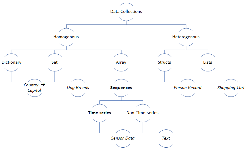
Data can also be composed together into “Collection” data types. Sets, Maps, Lists, and Arrays are examples of some collections. “Collections” with item order and homogeneity are called sequences. Movies and Text are sequences (arrays of images and words). In most cases, all data generated in a sequence is usually from the same source.

Sequences ordered by time are called time-series sequences, or just time-series for short. Sensor data that is generated periodically with a timestamp is an example of time-series data. Time-series data have properties like trend and seasonality that we will explore in a separate blog post. A camera (sensor) generates a time-series image data feed with a timestamp on every image. This feed is a time-series sequence.

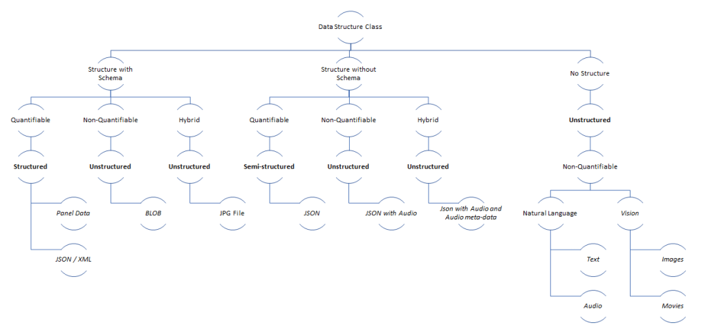
Some visuals will help to clarify this further:

Data by Measurement Class
Data by Structure (composition) Class

JSON and XML are data representations that come with or without schema. It’s incorrect to call all JSON documents semi-structured, as they might originate from a producer that uses well-defined schema and data typing rules.

Data Compositions

Hope this post helps to understand the “data measurement and composition vocabulary“. You can be strict or loose about classifying data by structure based on context—however, it’s critical to understand the measurement class.

Only measurable data generates insights.

After all that rant, let’s try to decipher “logs” data-type.

  1. “Performance Event Logs” generated by an application with fixed fields like {id: number, generated-by: application-name, method: method-name, time: time-since-epoch} is composed of quantifiable fields and constrained schema. So, it belongs to the “Structured Data” class.
  2. “Troubleshooting Logs” generated by an application with fields like {id: number, generated-by: application-name, timestamp: Date-time, log-type: <warn, info, error, debug>, text: BLOB, +application-specific-fields} is composed of quantifiable and non-quantifiable fields, without a constraining schema. Some applications may add additional fields like – API name, session-id, and user-id. Strictly, this is “unstructured” data due to the BLOB but loosely called “semi-structured” data.

Measurement-based data type classification and composition of types into structures do not convey semantics. We will cover semantics in our next blog!

Data Representation

Data Representation is a complex subject. People have built their careers in data representations, and some have lost their sleep. While the parent post refers to binary and non-binary data, the subject of data representations is more complex for a single blog post. If you are as old as me and lived through the data representation standardization, you will understand. If you are a millennial, you can reap the benefits of painful standardization of data structures. Semantic Data is still open for standardization.

What is Data?

Data is a collection of datum. Datum is singular, and Data is plural. In the computer language, “Data” is also widely (loosely) used as a singular.

A datum is a single piece of information (a single fact, a starting point for measurement). A character, a quantity, or a symbol on which computer operations (add, multiply, divide, reverse, flip) are applied. E.g., The character ‘H’ is a datum, and the string “Hello World” is data composed of different datum characters.

From now on, we will call ‘H’ and ‘Hello World’ as Data.

What are Data Types?

Data types are attributes of data that tell the computer the programmer’s intent to use the data. E.g., If the data type is a number, the programmer can add, multiply, and divide the data. If the data type is a character, then the programmer can compose the characters into strings. The operations add, multiply, and divide do not apply to characters.

Computers need to store, compute, and transfer different types of data.

Some common Data types are best described below that illustrate basic and composite data types:

Data TypesExamples
Characters and Symbols‘A’, ‘a’, ‘$’, ‘‘, ‘छ’
Digits0, 1, 2, 3, 4, 5, 6, 7, 8, 9
Integers (Signed and unsigned)-24, -191, 533, 322
Boolean (Binary)[True, False], [1, 0]
Floats (single precision)-4.5f
Doubles (double precision) -4.5d
Composite: Imaginary Numbersa + b*i
Composite: Strings“Heaven on Earth”
Composite: Arrays of Strings[‘Heaven’, ‘on’, ‘Earth’]
Composite: Maps (key-value){‘sad’: ‘:(‘, ‘happy’: ‘:)’}
Composite: Decimal (Fraction)22 / 7
Composite: Enumerations[Violet, Indigo, Blue, Green, Yellow, Orange, Red]
Table of Sample Data Types

What are Data Representations?

Logically, computers represent a datum by mapping it to a unique number and data as a sequence of numbers. This representation makes computing consistent – everything is a number. This mapping is called “Unicode.”

ExampleNumber
(Unicode code points)
HTMLComments
‘A’U+0041&#650x41 = 0d65
‘a’U+0061&#970x61 = 0d97
8U+0038&#560x38 = 0d56
‘ह’U+0939&#23610x939 = 0d2361
Sample Mapping Table

The numbers can themselves be represented in the base of 2, 8, 10, or 16. The human-readable number is base-10, whereas base-2 (binary), base-8 (octal), and base-16 (hexadecimal) are the other standard base systems. The Unicode code points (mappings) above are represented in hexadecimal.

Base-10Base-2Base-8Base-16
0d25
(2*10 + 5)
0b11001
(1*24 + 1* 23 + 0*22 + 0*21 + 1*20)
031
(3*81 + 1*80)
0x19
(1*161 + 9*160)
Base Conversion Table

Computers use base-2 (binary) to store, compute, and transfer data. Computers use base-2 because the electronic gates that make up the computers use binary inputs. Each storage cell in memory can store “one bit,” i.e., either a ‘0’ or a ‘1’. A group of 8 bits is a byte. The Arithmetic Logic Unit (ALU) uses a combination of AND, OR, NAND, XOR, NOR gates for mathematical operations (add, subtract, multiply, divide) on binary (base-2) representation of numbers. In modern memory systems (SSDs), each storage cell can store more than one bit of information. These are called MLCs (Multi-level cells). E.g., TLCs store 3 bits of information – or – 8 (23) stable states. This MLC helps to build fast, big, and cheap storage.

Historically, there have been many different character sets. E.g., ASCII for English, Windows-1252 (expanded ASCII) used by windows-95 systems to represent new characters and symbols. However, modern computers use the Unicode character set for (structural) interoperability between computer systems. The current Unicode (v.13) character set has 143,859 unique code points and can expand to 1,114,112 unique code points.

While all the characters in a character set can be mapped to numbers, precision point numbers (floats, doubles) are represented in the computers differently. They are represented as a composite of a sign, mantissa (significant), and exponent:

± (mantissa) * 2exponent

DecimalBinaryComment
1.51.11 * 20 + 1 * 2-1
33.25100001.011 * 25 + 0 * 24 + 0 * 23 + 0 * 22 + 0 * 21 + 1 * 20 + 0*2-1 + 1*2-2
Binary Representation of Decimal Numbers

The example below shows how 33.25 is converted to a float (single precision) representation – 1 sign bit, 8 exponent bits, 23 mantissa bits:

Convert 33.25 to Binary100001.01
Normalized Form(-1)0 * 1.0000101 * 25
[ (-1)s * mantissa * 2exponent ]
Convert exponent using biased notation
Represent decimal as binary
5 + 127 = 13210 = 1000 01002
Normalize the mantissa
Adjust to 23 bits by padding 0s
000 0101 0000 0000 0000 0000
Represent the 4 byte (32 bits)0100 0010 0000 0101 0000 0000 0000 0000
Floats (single precision) represented in 4 bytes

Some scientific computing requires double precision to handle the underflow/overflow issues of single precision. Double precision (64 bits) uses 1 sign bit, 11 exponent bits, and 52 mantissa bits. There are also long doubles that store 128 bits of information. The arithmetic operations (add, multiple) in the electronics are simplified using this binary representation.

Despite great computer precision, some software manages decimals as two separate fields (numerator and denominator) or (before . and after .) as multi-byte integers. These are called “Fraction” or “Decimal” data types and are usually used to store “money” where precision loss is unacceptable (i.e., 20.20 USD is 20 Dollars and 20 cents and not 20 Dollars and 0.199999999999 dollars).

What is Data Encoding?

Encoding is converting data represented by a sequence of numbers from the character set mapping into bits and bytes. The encoding process could be fixed width or variable width and is used for storage/transfer of data. Base64 encoding uses a fixed width (8 bits) encoding to represent 64 ASCII characters (A-Z, a-z, 0-9, special characters). UTF-8 encoding uses a variable width (1-4 bytes) encoding to represent Unicode character set.

TextBase64UTF-8
earthZWFydGg=01100101 01100001 01110010 01110100 01101000
éarthw6lhcnRo11000011 10101001 01100001 01110010 01110100 01101000
Base 64 encoding resulted in fixed-length representations, and UTF-8 resulted in variable-length representations. UTF-8 optimizes for the ASCII Character set and adds additional bytes for other code points. The character ‘ é ‘ is encoded into two bytes ( 11000011 10101001 ). This variable-length encoded sequence can be decoded because there is no conflict during the decoding process.

Base64 is usually used to convert binary data for media-safe data transfer. E.g., A modem/printer would interpret binary data differently (sometimes as control commands), so a base64 encoding is used to convert the data into ASCII to be media-safe. The Data is transferred as binary; however, since the bytes are ASCII (limited binary), the media/printer is not confused. If you observe, base64 has increased the number of bytes after the encoding. Earth (5 bytes) is encoded as ZWFydGg= (8 bytes). The Data is decoded back to binary at the receiver’s end. The example below shows the process:

1earth (40 bits)01100101 01100001 01110010 01110100 01101000
2Buffer to have bits in the multiples of 6 at byte boundaries (48 bits) [48 is 6 bytes and a multiple of 6]01100101 01100001 01110010 01110100 01101000 00000000
3Regroup into 6 bit bytes011001 010110 000101 110010 011101 000110 100000 000000
4Use Base64 table to map to text (see Wikipedia for base64 map)ZWFydGg=
5Convert to binary to send to store or transfer01011010 01010111 01000110 01111001 01100100 01000111 01100111 00111101

There are many different types of encodings – UTF-7, UTF-16, UTF-16BE, UTF-32, UCS-2, and many more.

What is Data Endianness?

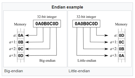
Endianness is the order of bytes in memory/storage or transfer. There are two primary types of Endianness: big-endian and little-endian. You might be interested in middle-endian (mixed-endian), and you can google that on your own.

As you can see in the diagram below, the computer may represent the data starting with the most significant byte (0x0A) or the least significant byte (0x0D).

Courtesy: Wikipedia

Most modern computers are little-endian when they store multi-byte data. Networks are consistently big-endian. So, little-endian memory dumps have to arrive at the network as big-endian.

Summary: There are many data types – basic (chars, integers, floats) and composite (arrays, decimals). Data is mapped to numbers using a universal character set (Unicode). This Data is represented as a sequence of code points in Unicode and converted into characters (or bits/bytes) using an encoding process. The encoding process can be fixed-length (E.g., Base64, UTF-32) or variable length (UTF-8, UTF-16). Computers can be little or big-endian. Modern CISC computers (Intel x86) are little-endian, and RISC computers (ARM Processors) are big-endian. Networks are always big-endian.

Tips/Tricks: Stick to Unicode character set and UTF-8 encoding scheme. Use Base64 to transfer data to be media-safe (e.g., base64 encoding of strings in HTTP URLs to make them URL-safe). Using a modern programming language (E.g., Java) abstracts you from the Endianness. If you are an embedded engineer programming in C, you need to develop code to be Endianness safe (e.g., type casts and memcpy).

Even with all this structure, we cannot convey meaning (semantics). An ‘A’ for the computer is always U+0041. If the programmer wants to transfer ‘A,’ ‘A,’ or ‘A,’ more information is encoded for the receiver to interpret. More on that in future blogs.

This one was too long even for me!

Data about Data

As a Data Engineer, I want to be able to understand the data vocabulary, so that I can communicate about the data more meaningfully and find tools to deal with the data for computingData Engineer

Let’s start with this: Binary Data, Non-binary Data, Structured Data, Unstructured Data, Semi-structured Data, Panel Data, Image Data, Text Data, Audio Data, Categorical Data, Discreet Data, Continuous Data, Ordinal Data, Numerical Data, Nominal Data, Interval Data, Sequence Data, Time-series Data, Data Transformation, Data Extraction, Data Load, High Volume Data, High Velocity Data, Streaming Data, Batch Data, Data Variety, Data Veracity, Data Value, Data Trends, Data Seasonality, Data Correlation, Data Noise, Data Indexes, Data Schema, BIG Data, JSON Data, Document Data, Relational Data, Graph Data, Spatial Data, Multi-dimensional Data, BLOCK Data, Clean Data, Dirty Data, Data Augmentation, Data Imputation, Data Model, Object (Blob) Data, Key-value Data, Data Mapping, Data Filtering, Data Aggregation, Data Lake, Data Mart, Data Warehouse, Database, Data Lakehouse, Data Quality, Data Catalog, Data Source, Data Sink, Data Masking, Data Privacy

Now let’s go here: High volume time-series unstructured image data, High velocity semi-structured data with trends and seasonality without correlation, High volume Image data with Pexels Data source masked and stored in Data Lake as the Data Sink.

The vocabulary is daunting for a beginner. These 10 categories (ways of bucketizing) would be a good place to start:

  1. Data Representation for Computing: How is Data Represented in a Computer?
    • Binary Data, Non-binary Data
  2. Data Structure & Semantics: How well is the data structured?
    • Structured Data, Unstructured Data, Semi-structured Data
    • Sequence Data, Time-series Data
    • Panel Data
    • Image Data, Text Data, Audio Data
  3. Data Measurement Scale: How can data be reasoned with and measured?
    • Categorial Data, Nominal Data, Ordinal Data
    • Discreet Data, Interval Data, Numerical Data, Continuous Data
  4. Data Processing: How is the data processed?
    • Streaming Data, Batch Data
    • Data Filtering, Data Mapping, Data Aggregation
    • Clean Data, Dirty Data
    • Data Transformation, Data Extraction, Data Load
    • Data Augmentation, Data Imputation
  5. Data Attributes: How can data be broadly characterized?
    • Velocity, Volume, Veracity, Value, Variety
  6. Data Patterns: What are the patterns found in data?
    • Time-series Data Patterns: Trends, Seasonality, Correlation, Noise
  7. Data Relations: What are the relationships within data?
    • Relational Data, Graph Data, Document Data (Key-value Data, JSON Data)
    • Multi-dimensional Data, Spatial Data
  8. Data Storage Types:
    • Block Data, Object (Blob) Data
  9. Data Management Systems:
    • Filesystem, Database, Data Lake, Data Mart, Data Warehouse, Data Lakehouse
    • Data Indexes
  10. Data Governance, Security, Privacy:
    • Data Catalog, Data Quality, Data Schema, Data Model
    • Data Masking, Data Privacy

More blogs to deep dive into each category and the challenges involved. Let’s peel this onion.